Density Estimation in Statistical Analysis
Density estimation is a vital technique in statistics that reconstructs the probability density function (PDF) of a random variable from observed data. It serves a fundamental role in analyzing the distribution’s characteristics, such as modality and skewness, and can be applied in various tasks, including classification and anomaly detection.
Key Concepts
-
Probability Distribution: A random variable ( X ) can be characterized by its cumulative distribution function (CDF), ( F(x) ).
- Discrete Case: The probability mass function (PMF) can be derived from the CDF.
- Continuous Case: The PDF is obtained by differentiating the CDF, ( p(x) = F'(x) ).
-
Need for Density Estimation: Direct estimation of the PDF from a sample is not straightforward, especially when ( X ) is continuous. While the CDF can be constructed from empirical data, differentiating this estimate to obtain the PDF leads to inaccuracies.
- Types of Density Estimation:
- Parametric: Assumes that data follows a known distribution characterized by parameters (e.g., normal distribution).
- Non-parametric: Makes fewer assumptions about the underlying distribution and estimates the density directly from the data.
Focus of Discussion
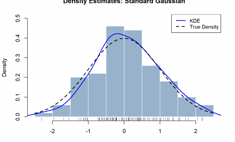
This article primarily explores two non-parametric methods for density estimation: Histograms and Kernel Density Estimators (KDEs). Each method has its own benefits and drawbacks, impacting its effectiveness in estimating a random variable’s true density.
Histograms
Overview
Histograms are a straightforward approach where the data range is divided into equal-length bins, and the density is determined by the proportion of data points within each bin.
Density Estimate Formula:
For a point ( x ) in bin ( beta_l ), the density estimate is given by the formula that normalizes the frequency of observations in the bin.
Theoretical Properties
- Non-negativity: Histograms produce non-negative density estimates.
- Normalization: The area under the histogram integrates to 1, satisfying the properties of a probability density function.
Mean Squared Error (MSE):
The accuracy of histograms can be assessed using MSE, which breaks down into bias and variance.
- Bias: As the bin width ( h ) approaches 0, histogram estimates become unbiased.
- Variance: As ( h ) increases, variance increases, leading to a trade-off:
- Smaller bin widths reduce bias but increase variance due to higher sensitivity to data fluctuations.
- Larger bin widths smooth out random variations but may obscure details about the data distribution.
Conclusion
Density estimation is a crucial statistical tool with various applications. By understanding histograms and KDEs’ advantages and challenges, you’re better equipped to analyze data distributions and apply these techniques effectively. This knowledge can pave the way for more complex statistical analyses and models.